The already presented demonstration example initially was preset with any non-optimal employment matrix ac. We can now specify the associated optimal matrix and calculate the other secondary parameters to evaluate the result.

In the following values, all values belonging to the optimal solution are marked with the index "optimal" in order to distinguish them from the other values of the non-optimal employment matrix already given above, which will be shown again for comparison.

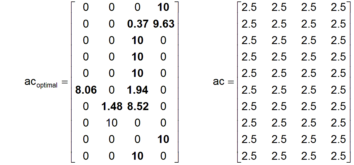
The optimal employment matrix ac_optimal has the values

As a reminder for the interpretation of the employment matrix: The first line of ac_optimal means that all 10 workers in the first performance group are employed in the fourth occupation.

The standardized productivities pn, the mean productivities pm_optimal and the productivity increase factors fp_optimal have the values

pn            = [ 2.45  2.00  1.65  2.30 ]   º   pn   = [ 2.45  2.00  1.65  2.30 ]

pmoptimal = [ 8.00  5.61  1.90  4.35 ]        pm = [ 2.45  2.00  1.65  2.30 ]

fpoptimal   = [ 3.26  2.81  1.15  1.89 ]        fp   = [ 1.00  1.00  1.00  1.00 ]

It is shown that the optimization in our example has in some cases resulted in considerable increases of productivity in several professions. It is lowest in the professions in which a strong selection is not possible due to the high demand for workers, as can be seen in occupation j3=3..

The overall societal work performance d_optimal, the included needs-conform proportions db_optimal and the factors fb_optimal of needs-conformity have the values

doptimal   = [ 64.44  64.44  96.67  128.89 ]     d    = [ 61.25  50.00  41.25  57.50 ]

dboptimal = [ 64.44  64.44  96.67  128.89 ]     db = [ 27.50  27.50  41.25  55,00 ]

fboptimal  = [   1.00     1.00     1.00     1.00 ]     fb  = [    0.45    0.55    1.00    0.96 ]

As expected in the optimal solution applies d_optimal = db_optimal, that means all workers are involved in all professions in the overall societal needs-based work performance. This is a necessary but not a sufficient condition for actually achieving the optimum.

At last, two complex evaluation parameters should be added. These are the factor fbg of the needs-conformity of the overall societal work performance and the factor fg of the overall societal increase in performance

fbgoptimal = 1.00           fbg = 0.74

fgoptimal   = 1.73           fg   = 0.74

As expected, the factor fbg_optimal equals one, since all fb_optimal already equaled the values one.

The most important evaluation factor fg_optimal tells us that by the optimal employment matrix ac_optimal, which means by an optimal employment policy compared to our arbitrary initial employment matrix ac with fg=0.74, an increase in the overall societal performance of 2.33 is possible.

db_optimal /db = fg_optimal /fg=1.73/0,74=2.33

This increase in performance is only based on the optimal use of the workforce, in which everyone does what one can do best relative to others, taking into account the needs of society as a whole. Nobody has to exert themselve more than normal, because normal exertion for all workers in every profession was assumed within the matrix p of individual productivities.

The fact that this solution really represents the optimum is not quite apparent in the results. Only the simplex algorithm guarantees that it is the optimum. In rare cases there may be some other employment matrices that lead to the same increase in performance.