6.2 Test calculations with the demonstration example
A test calculation has already been executed with the demonstration example mentioned earlier. In addition to the predefined time-invariant parameters "productivity matrix p", "productivity group sizes ap" and "needs-based performance structure db0 or dbn" the non-optimal employment matrix ac was assumed as the initial parameter. A vector Is of piece wages, which serve as initial values has to be added to this data record. This vector ls of piece wages does not have to be optimal since self-optimization is expected within the simulation calculation, too. An arbitrary starting vector was determined by
lsi4=0 = [ 1 1 1 1]
Furthermore, the empirical factors of the fluctuation rate r1 and the speed of price adjustment r2 must be given. It was assumed
r1 = 0.3 r2 = 0.3
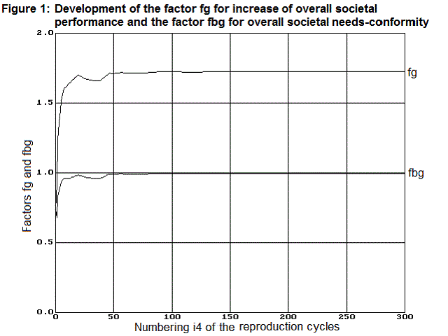
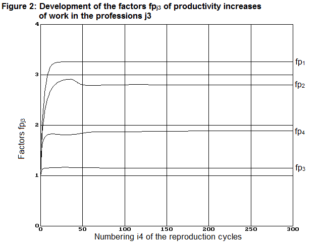
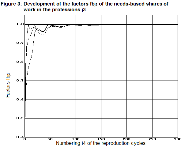
Over n4=300 reproduction cycles have been calculated. In our example the model of the labor market actually converges to the optimal employment matrix acoptimal, as we have already calculated in another way. After approximately 100 reproduction cycles the maximum increase in performance and the needs-based work performance are achieved. The maximum increase in performance is represented using the factor fg (and separately using the factors fpj3). The needs-based work performance is represented using the factor fbg (and separately using the factors fbj3).
fgn4=0 = 0.74 fpn4=0 =[1.00 1.00 1.00 1.00]
fgn4=300 = 1.73 fpn4=300=[3.26 2.81 1.15 1.89]
and
fbgn4=0 = 0.74 fbn4=0 =[0.45 0.55 1.00 0.96]
fbgn4=300= 1.00 fbn4=300=[1.00 1.00 1.00 1.00]
In Figures 1 to 3 diagrams demonstrate these factors in their time course from n4= 1 to 300 and thus demonstrate the convergence behaviour of the model by this example.
The piece wages lsj3 also converge to optimal values. Here, however, the optimal values are only reached after approx. 150 reproduction cycles as can be seen in Figure 4.
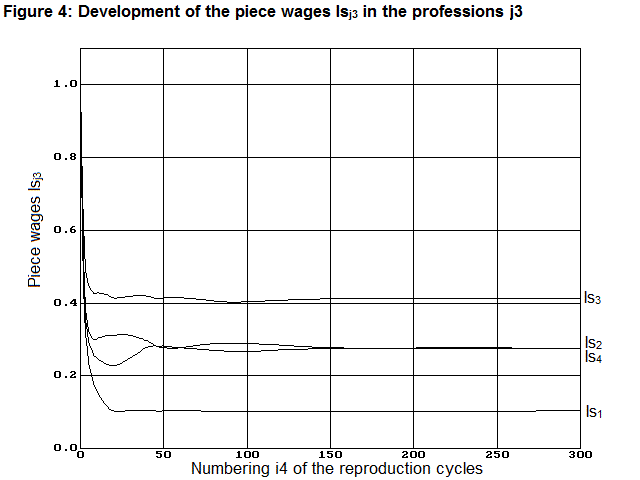
After 300 reproduction cycles, the piece wages lsi4=300 had reached the following almost optimal values.
lsopt » lsi4=300 = [0.103 0.276 0.414 0.276]
The simulation program also provides the matrix of the individual wages li4=300 after 300 reproduction cycles. Together with the employment matrixaci4=300 » acoptimal, which corresponds to the optimal employment matrix, it shows which wages the workers actually receive in their current professions and also which wages they are (would be) receiving in other professions at the same time. The realized wages are highlighted in bold in the matrix li4=300 given below. In addition the associated employment matrix is also given here.
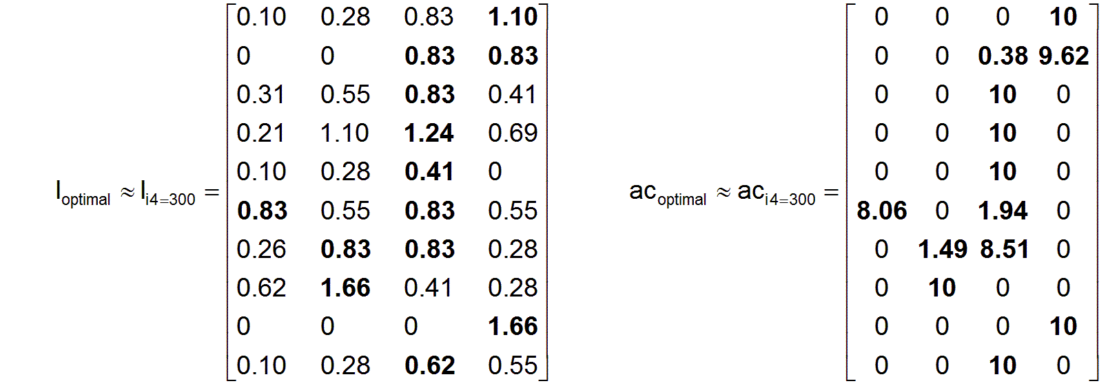
The remarkable result shows that there is actually an optimal system of piece wages, which ensures that all workers in the profession in which they are working in the interests of an overall societal maximum needs-based work actually receive the highest individual wages without exception. Accordingly, they should endeavor to work precisely in the respective profession, given they are sufficiently informed. What is also interesting about the result is that the system has led to optimal unit wages and thus to optimal individual wages in a self-optimizing way simply by a very simple principle of wage adjustment according to supply and demand.
Return Go on